


Every time ChatGPT writes a sentence, Claude answers a question, or Gemini summarizes a document, hundreds of billions of mathematical operations fire in sequence. Numbers multiply through matrices. Activation functions decide which signals pass and which die. Attention heads compute relevance scores across thousands of tokens. And the output — a single word — gets appended to the sequence before the entire process repeats.
The result feels like understanding. It feels like intelligence. But the underlying mechanism is deceptively simple: predict the next token.
That simplicity is what makes large language models so fascinating — and so difficult to explain. How does a system trained on nothing but next-word prediction learn to write code, solve differential equations, and debate philosophy? How do 200,000-token vocabularies and trillions of parameters combine to produce something that passes medical licensing exams and writes production-ready software?
This article answers those questions. We will trace the full arc — from the first artificial neuron in 1943 to the transformer architecture that powers every major LLM in 2026 — and explain each piece in plain language. No PhD required.
TL;DR: Large language models work by predicting the next token in a sequence using the transformer architecture. They are trained on trillions of text examples through backpropagation, developing emergent capabilities like reasoning, coding, and conversation at scale. Every major model — GPT, Claude, Gemini — uses this same fundamental approach. Build with frontier LLMs in Taskade →
💡 Before you start... Explore these related deep dives:
- What Is Agentic AI? — How LLMs become autonomous agents
- What Are AI Agents? — The anatomy of intelligent systems
- What Is Generative AI? — The broader category LLMs belong to
- OpenAI and ChatGPT: The Full History — From GPT-1 to today's frontier models
- Anthropic and Claude: The Full History — Safety-first AI research
🧠 How Do Large Language Models Work?
Large language models work by predicting the next token in a sequence, trained on trillions of examples of human text. A token is a word or sub-word unit — the word "understanding" might be split into "under" + "stand" + "ing." The model sees a sequence of tokens, computes probability distributions over its entire vocabulary (typically 100,000-200,000 tokens), and selects the most likely continuation. This process repeats, one token at a time, until the response is complete.
The shocking part is that this is all there is. Every capability you have seen from ChatGPT, Claude, or Gemini — writing essays, debugging code, translating languages, reasoning through logic puzzles — emerges from next-token prediction at sufficient scale.
Geoffrey Hinton, often called the "godfather of deep learning," built one of the first neural language models in 1985. It had a tiny vocabulary and could barely complete simple sentences. Four decades later, the same core idea — predicting the next element in a sequence — drives models with trillions of parameters that can pass the bar exam.
The difference is not the idea. The difference is scale — and a single architectural innovation called the transformer.
Evolution of Language Models:
| Model | Year | Parameters | Key Capability |
|---|---|---|---|
| Hinton's LM | 1985 | ~1,000 | Simple word prediction |
| GPT-2 | 2019 | 1.5 billion | Coherent paragraphs |
| GPT-3 | 2020 | 175 billion | Few-shot learning, reasoning |
| GPT-4 | 2023 | ~1.8 trillion (est.) | Professional-exam performance |
| Frontier model (OpenAI, 2025) | 2025 | ~2 trillion (est.) | Codeforces top-6, extended reasoning |
| Frontier model (Anthropic, 2025) | 2025 | Undisclosed | Deep reasoning, 200K context |
Every model in this table is built on the same foundation: artificial neurons, backpropagation, and the transformer architecture. Let us examine each piece.
⚡ The Artificial Neuron: Where It All Begins
The artificial neuron is the smallest unit of computation in a neural network. In 1943, neurophysiologist Warren McCulloch and logician Walter Pitts published a paper proposing a mathematical model of biological neurons: a unit that takes multiple inputs, multiplies each by a weight, sums the results, and fires if the total exceeds a threshold.
The biological inspiration is direct. The human brain contains approximately 86 billion neurons connected by roughly 100 trillion synapses. Each biological neuron receives electrical signals from thousands of other neurons, integrates those signals, and either fires (sending a signal onward) or stays silent. McCulloch and Pitts showed this process could be represented mathematically.
     Inputs      Weights     Neuron
    ┌──────┐    ┌──────┐   ┌────────────┐
    │ x₁   │───│ w₁   │──▶│            │
    │ x₂   │───│ w₂   │──▶│  Σ(xᵢwᵢ)  │──▶ Output
    │ x₃   │───│ w₃   │──▶│  + bias    │   (0 or 1)
    └──────┘    └──────┘   └────────────┘
                            if sum > threshold → fire
In 1949, Canadian psychologist Donald Hebb proposed a learning rule that became foundational: "Neurons that fire together, wire together." When two connected neurons activate simultaneously, the connection between them strengthens. This became the theoretical basis for how artificial neural networks learn — by adjusting the weights between connected units.
Frank Rosenblatt's Perceptron (1958) was the first practical implementation. Built at Cornell, the Perceptron was a physical machine (not just math on paper) that learned to recognize simple shapes. It took pixel inputs, multiplied them by adjustable weights, and classified images as belonging to one category or another. The machine learned by adjusting its weights when it made mistakes. The New York Times ran the headline: "New Navy Device Learns by Doing."
But the Perceptron had a fundamental limitation. It could only learn linearly separable patterns — problems where you can draw a straight line between categories. In 1969, Marvin Minsky and Seymour Papert published Perceptrons, a book proving mathematically that single-layer networks could not solve a basic logic problem called XOR (exclusive or). The implication was devastating: neural networks were fundamentally limited.
Funding dried up. Researchers abandoned the field. The first AI winter had begun.
The solution required stacking neurons into multiple layers — a "deep" network — and finding a way to train every layer simultaneously. That would take another 17 years.
🔗 Backpropagation: Teaching Networks to Learn
Backpropagation is the algorithm that enabled deep learning by solving the credit assignment problem: when a multi-layer network produces a wrong answer, how do you determine which weights in which layers contributed to the error? Published by David Rumelhart, Ronald Williams, and Geoffrey Hinton in 1986, backpropagation computes the gradient of the error with respect to each weight in the network, layer by layer, from output back to input.
The algorithm works in four steps:
- Forward pass: Input flows through the network, layer by layer, producing an output
- Error computation: The output is compared to the correct answer, producing a loss value
- Backward pass: The error signal propagates backwards through each layer, computing how much each weight contributed to the error (using the chain rule of calculus)
- Weight update: Each weight is nudged in the direction that reduces the error
Before backpropagation, training a multi-layer network was considered impossible. You could train single-layer networks (Perceptrons) by directly comparing output to the correct answer, but with multiple hidden layers between input and output, there was no way to know which interior weights to adjust. In 1959, Widrow and Hoff at Stanford came agonizingly close — their LMS algorithm used calculus to compute gradients for single-layer networks. But the binary step activation function (output 1 or 0) killed the gradient at layer boundaries: its derivative is zero everywhere. The fix was replacing the step function with a smooth sigmoid curve, but nobody made this connection for 27 years.
Backpropagation solved this by applying the chain rule of calculus recursively — through sigmoid activations that kept the gradient alive across layers. If the output error depends on layer 3's activations, and layer 3's activations depend on layer 2's weights, then you can compute exactly how much each weight in layer 2 contributed to the final error. Apply this recursively through all layers, and you can train networks of arbitrary depth.
The impact cannot be overstated. Every major advancement in AI since 1986 relies on backpropagation. The algorithm that trains ChatGPT is fundamentally the same one Hinton published four decades ago — applied at incomprehensibly larger scale.
After the 1986 paper, neural networks experienced a renaissance. Researchers trained networks for speech recognition, handwriting recognition, and simple language tasks. But hardware limitations kept networks small. The true explosion would not come until the 2010s, when GPUs made it possible to train networks with millions, then billions, then trillions of parameters.
The next breakthrough was not about learning — it was about architecture. How do you structure a neural network to understand language?
But before we reach the transformer, there are two hidden chapters in this story. The first is about the road not taken — the symbolic approach that dominated AI for decades before neural networks won. The second connects neural networks not to computer science, but to physics.
The Road Not Taken: Symbolic AI and the Common Sense Problem
While Rosenblatt's perceptron languished during the AI winters, a different approach to intelligence thrived. In 1956, John McCarthy coined the term "artificial intelligence" at the Dartmouth Conference and invented LISP — a programming language designed specifically for symbolic reasoning. McCarthy and the symbolic AI camp believed intelligence was about manipulating symbols according to logical rules: if A implies B, and B implies C, then A implies C.
By 1984, this philosophy had produced an entire industry. On a landmark episode of The Computer Chronicles, McCarthy appeared alongside Nils Nilsson (Stanford) and Edward Feigenbaum to showcase the state of the art: expert systems. MYCIN diagnosed 20 infectious diseases using 300 hand-coded rules. XCON saved Digital Equipment Corporation $40 million per year configuring computer orders. Feigenbaum coined the term "knowledge engineering" — the process of extracting expertise from human specialists and encoding it into rules.
But McCarthy, even as the symbolic approach peaked, identified its fatal flaw: these systems had no common sense. A medical expert system could diagnose a rare blood infection but could not understand that patients have bodies, live in a world with gravity, and might be afraid. The "things everybody knows" — the vast ocean of implicit knowledge humans navigate unconsciously — could not be formalized into rules.
THE TWO ROADS TO INTELLIGENCE  SYMBOLIC AI (McCarthy, Minsky)       NEURAL NETWORKS (Rosenblatt, Hinton)
  ┌─────────────────────┐              ┌─────────────────────┐
  │ Intelligence =      │              │ Intelligence =      │
  │ symbol manipulation │              │ pattern learning    │
  │                     │              │                     │
  │ Hand-coded rules    │              │ Learned weights     │
  │ Logic, LISP         │              │ Statistics, calculus│
  │ Explicit knowledge  │              │ Implicit knowledge  │
  │                     │              │                     │
  │ Strength: precise   │              │ Strength: general   │
  │ Weakness: brittle   │              │ Weakness: opaque    │
  └──────────┬──────────┘              └──────────┬──────────┘
             │                                    │
             └──────────────┬─────────────────────┘
                            ▼
             ┌──────────────────────────┐
             │  TRANSFORMERS (2017)     │
             │  Attention = structured  │
             │  pattern learning        │
             │  The synthesis           │
             └──────────────────────────┘
The irony: the symbolic approach dominated the 1980s while neural networks were dismissed as a dead end. By the 2010s, the positions reversed completely. And modern transformers — with their attention mechanisms (structured, symbolic-like selection) operating on learned representations (connectionist foundations) — turned out to be the synthesis of both traditions. McCarthy's common sense problem remains the hardest unsolved challenge in AI, but LLMs approximate it through brute-force statistical learning at a scale McCarthy could never have imagined.
Now for the second hidden chapter — the one that won a Nobel Prize.
🧲 The Physics of Neural Networks: From Magnets to Minds
On October 8, 2024, John Hopfield and Geoffrey Hinton received the Nobel Prize in Physics — not Chemistry, not the Turing Award, but Physics — for their contributions to artificial neural networks. The award surprised many in the AI community. It should not have. The deepest roots of modern AI are planted in statistical mechanics, the physics of magnets, and the mathematics of energy landscapes.
The connection starts in 1920, when German physicist Wilhelm Lenz posed a problem to his student Ernst Ising: model how a block of iron becomes a permanent magnet. The Ising model imagined a grid of atoms, each carrying a tiny magnetic spin — either up or down. Two rules governed the system:
- Temperature causes random spin flips (noise)
- Adjacent spins tend to align because aligned configurations have lower energy and are more stable
As the system evolves, magnetic domains emerge — regions where nearby spins point the same direction. Add an external magnetic field, and the entire block aligns into a large-scale magnet. The key insight: the system naturally rolls toward lower-energy, more stable configurations, like a marble settling into a valley.
THE ISING MODEL → HOPFIELD NETWORK → MODERN AIPhysics (1920)              AI (1982)                  AI (2026)
┌─────────────────┐   ┌─────────────────┐   ┌─────────────────────┐
│ Atoms with spins│   │ Neurons (on/off)│   │ Transformer layers  │
│ up ↑ or down ↓  │   │ activated or not│   │ billions of params  │
├─────────────────┤   ├─────────────────┤   ├─────────────────────┤
│ Adjacent spins  │   │ Weighted         │   │ Attention heads     │
│ tend to align   │   │ connections      │   │ compute relevance   │
├─────────────────┤   ├─────────────────┤   ├─────────────────────┤
│ System minimizes│   │ Network finds   │   │ Training minimizes  │
│ energy          │   │ stored patterns │   │ loss function       │
├─────────────────┤   ├─────────────────┤   ├─────────────────────┤
│ Domains emerge  │   │ Memories emerge │   │ Capabilities emerge │
└─────────────────┘   └─────────────────┘   └─────────────────────┘
        ▼                     ▼                        ▼
  Ferromagnetism      Associative Memory       Language, Reasoning,
                                               Code, Math, Agents
In 1982, American physicist John Hopfield realized the Ising model could be repurposed as a memory machine. Instead of atoms with spins, the Hopfield network used artificial neurons that were either active or inactive. Instead of physical proximity governing interactions, each connection between neurons carried a weight — a number determining how much one neuron influences another.
The genius was in the energy landscape. By carefully setting the weights, Hopfield could sculpt valleys in the network's energy surface around specific patterns. When you fed the network a noisy or incomplete pattern, it would naturally roll downhill toward the nearest valley — the nearest stored memory. The network "remembered" by relaxing into a memorized state.
Geoffrey Hinton took Hopfield's idea further. His Boltzmann machine (1985) — named after the physicist Ludwig Boltzmann, father of statistical mechanics — added probabilistic learning to the network. Hinton showed that neural networks could be trained using concepts borrowed directly from thermodynamics: temperature, energy, entropy, equilibrium. The training process resembled a physical system cooling down and crystallizing into an ordered state — a technique called simulated annealing.
This is why Hinton won a Nobel Prize in Physics, not Computer Science. The mathematical frameworks are the same. A neural network minimizing its loss function during training is doing the same math as a physical system minimizing its energy. The gradients that backpropagation computes are analogous to the forces that push a physical system toward equilibrium.
AlexNet: The Scale Tipping Point (2012)
The physics-inspired ideas of Hopfield and Hinton remained niche for decades — brilliant but computationally impractical. Then, in 2012, everything changed.
Hinton's student Ilya Sutskever (who would later co-found OpenAI) and Alex Krizhevsky built AlexNet — a deep convolutional neural network that stunned the computer vision community by winning the ImageNet challenge by a massive margin. The architecture was not new. The ideas were from the 1980s and 1990s. What was new was scale: 1.3 million training images and Nvidia GPUs providing 10,000x more compute than previous attempts.
| Model | Year | Parameters | Compute (relative) | What Changed |
|---|---|---|---|---|
| LeNet-5 (LeCun) | 1998 | 60,000 | 1x | Handwritten digits |
| AlexNet | 2012 | 60 million | ~10,000x | ImageNet, GPUs |
| GPT-3 | 2020 | 175 billion | ~10,000,000x | Language understanding |
| Frontier LLMs | 2025 | ~2 trillion | ~100,000,000x | Multi-hour autonomous tasks |
The pattern is clear: every major AI breakthrough is the same ideas, scaled by 3-4 orders of magnitude. AlexNet was Rosenblatt's Perceptron scaled up. GPT-3 was AlexNet's deep learning scaled up. The physics has not changed since Hopfield. The scale has.
What made AlexNet revelatory was what researchers found when they looked inside. The first layer had learned to detect edges and color blobs — visual primitives that neuroscientists had identified in biological visual cortex decades earlier. Deeper layers combined these into corners, textures, and eventually high-level concepts like faces — despite never being told what a face is. The network organized visual information into a hierarchy of increasing abstraction, mirroring the structure of the biological brain.
Even more striking: the second-to-last layer of AlexNet produced a 4,096-dimensional embedding vector for each image. Images of elephants clustered near other elephants in this high-dimensional space. Images of guitars clustered near guitars. The pixel values between these images could be completely different, but the model had learned abstract representations where similar concepts are geometrically close. This is the same embedding principle that powers every modern LLM — words with similar meanings cluster in embedding space, just as AlexNet's images clustered by concept.
Researchers later created activation atlases — 2D projections of these high-dimensional spaces — that let you visually walk through how a neural network organizes the world. Moving across the atlas, you see smooth transitions from zebras to tigers to leopards to rabbits. It is a map of the model's learned understanding, and it is hauntingly beautiful.
The Quantum Connection
In 2020, researchers at the NSF AI Institute for Artificial Intelligence and Fundamental Interactions (IAIFI) discovered an unexpected correspondence: the statistics of very wide neural networks behave identically to quantum field theory — the physics framework describing how subatomic particles interact.
A neural network maps input values to output values — it acts as a mathematical field. When you randomize the network's weights and observe the distribution of outputs, something remarkable happens: as the network grows wider, the output distribution converges to a Gaussian (bell curve). This is the same distribution that describes a free quantum field — one without particle interactions.
In real neural networks (which are not infinitely wide), the distribution deviates slightly from Gaussian. These deviations are mathematically analogous to particle interactions in quantum field theory. Physicists can even use Feynman diagrams — the visual calculus of particle physics — to study how information propagates through neural networks.
This is not a metaphor. The math is identical. Neural networks and quantum fields are described by the same equations. As the IAIFI researchers put it: understanding neural networks may require the same tools physicists use to understand the universe itself.
The implications flow both ways. AI is now used in experimental physics to denoise gravitational wave signals, analyze particle collision data, predict protein structures (the 2024 Nobel Prize in Chemistry went to AlphaFold), map dark matter in galaxies, and explore string theory. And physics provides the mathematical tools — energy landscapes, phase transitions, field theory — to understand how AI actually works.
The line between physics and AI is not blurring. It was never there.
🏗️ The Transformer Architecture
The transformer is the neural network architecture that powers every major large language model in 2026. Introduced in the 2017 paper "Attention Is All You Need" by Ashish Vaswani and colleagues at Google, it replaced the sequential processing of previous architectures with parallel self-attention, making it possible to train on massive datasets efficiently.
Before transformers, the dominant architecture for language was the Recurrent Neural Network (RNN) and its variants (LSTM, GRU). RNNs processed text one word at a time, maintaining a hidden state that carried information forward. This sequential processing had two critical problems:
- Slow training: You could not parallelize computation because each step depended on the previous step
- Vanishing context: By the time the network reached the 500th word, information about the 1st word had been diluted through hundreds of sequential operations
The transformer solved both problems simultaneously. But the solution introduced its own constraint: self-attention is O(n²) in sequence length — every token attends to every other token. This quadratic cost is why context windows are expensive, why longer prompts cost more, and why architectural decisions (not just code) determine whether an AI system is practical. Understanding algorithmic complexity matters more than ever — not because you'll implement attention from scratch, but because the performance implications shape what you can build.
How a Transformer Processes Text:
Step 1 — Tokenization. Raw text is split into tokens. The sentence "Understanding transformers is fascinating" might become ["Under", "standing", " transform", "ers", " is", " fascinating"]. Modern tokenizers like BPE (Byte Pair Encoding) build a vocabulary of 100,000-200,000 sub-word units that balance vocabulary size against token count.
Step 2 — Embedding. Each token is converted into a dense vector — a list of numbers (typically 4,096-12,288 dimensions) that represents the token's meaning. Initially, these embeddings are random. Through training, tokens with similar meanings develop similar vectors. The embedding for "king" minus "man" plus "woman" produces a vector close to "queen" — the model learns semantic relationships as geometry.
Step 3 — Positional Encoding. Because the transformer processes all tokens simultaneously (not sequentially), it needs a way to know word order. Positional encodings add information about each token's position in the sequence, so the model can distinguish "the dog bit the man" from "the man bit the dog."
Step 4 — Self-Attention. Each token attends to every other token in the sequence, computing relevance scores. This is where the transformer's power lives. (We dedicate the next section to this mechanism.)
Step 5 — Feed-Forward Network. After attention, each token's representation passes through a feed-forward neural network (two linear layers with a nonlinear activation function like ReLU or GELU). This is where the model does its "thinking" — transforming the attention-enriched representations.
Step 6 — Repeat. Steps 4 and 5 constitute one transformer "block." Modern LLMs stack 32 to 128 blocks, each refining the representation. Early layers capture syntax and grammar; later layers capture semantics, logic, and reasoning.
Step 7 — Output. The final representation of the last token is projected back into the vocabulary space, producing a probability distribution over all possible next tokens. The model selects the most probable token (or samples from the distribution with some randomness, controlled by a "temperature" parameter).
┌─────────────────────────────────────────┐
│           TRANSFORMER BLOCK             │
│                                         │
│  ┌─────────────────────────────────┐   │
│  │     Multi-Head Attention        │   │
│  │  ┌─────┐ ┌─────┐ ┌─────┐      │   │
│  │  │ Q·K │ │ Q·K │ │ Q·K │      │   │
│  │  │ ──▶ │ │ ──▶ │ │ ──▶ │      │   │
│  │  │  V  │ │  V  │ │  V  │      │   │
│  │  └─────┘ └─────┘ └─────┘      │   │
│  └─────────────────────────────────┘   │
│              ↓ + Residual               │
│  ┌─────────────────────────────────┐   │
│  │    Feed-Forward Network         │   │
│  │    (2 linear layers + ReLU)     │   │
│  └─────────────────────────────────┘   │
│              ↓ + Residual               │
└─────────────────────────────────────────┘
         × N layers (96+ in frontier models)
The "Attention Is All You Need" paper has been cited over 130,000 times — making it one of the most influential computer science papers ever published. Its core insight — that you do not need recurrence or convolution to model language, just attention — unlocked the era of large language models.
By the Numbers: What 175 Billion Parameters Actually Look Like
It is easy to get lost in "175 billion parameters" without a sense of where those numbers live. GPT-3 — still the cleanest reference point because OpenAI published its dimensions before the modern era of secrecy — distributes its weights across just under 28,000 distinct matrices, organized into eight functional categories (embedding, unembedding, query, key, value, output projection, and two feed-forward matrices per block). Almost every operation inside the model reduces to matrix-vector multiplication: the data flowing through is one column of numbers per token, and the weights are giant rectangles of tunable parameters that transform those columns.
The concrete shapes are worth memorizing because they recur across nearly every modern LLM:
| Quantity | GPT-3 value | What it controls |
|---|---|---|
| Vocabulary size | 50,257 tokens | How text is chunked before embedding |
| Embedding dimension | 12,288 | How much "meaning" each token vector can carry |
| Context length | 2,048 tokens | How much text the model can attend to at once |
| Transformer blocks | 96 | How many attention + feed-forward refinement passes |
| Attention heads per block | 96 | How many simultaneous relevance perspectives |
| Embedding matrix (W_E) | 50,257 × 12,288 | ~617M params — turns tokens into vectors |
| Unembedding matrix (W_U) | 12,288 × 50,257 | ~617M params — turns the final vector back into a probability distribution |
That last row matters more than it looks. At the very end of the network, only the last vector in the sequence is multiplied by the unembedding matrix to produce the next-token distribution. Every other vector in the final layer is "wasted" at inference time — but during training, every position predicts its own next token in parallel, which is what makes the math tractable on trillion-token corpora.
Embeddings Are Geometry, Not Lookups
The reason king − man + woman ≈ queen works is not a trick. When a transformer is trained, it discovers that the most efficient way to compress meaning into 12,288 numbers is to make directions in the embedding space carry semantic content. Gender becomes one axis. Plurality becomes another. "Italian-ness" becomes another. Nobody designs these axes — they fall out of gradient descent because they reduce loss.
This is also why the dot product shows up everywhere inside attention. The dot product of two vectors is large and positive when they point the same way, zero when they are perpendicular, and negative when they oppose — so it is a natural similarity score. When a Query vector dot-products with a Key vector, the model is literally asking "how aligned are these two meanings in the learned geometry?" Every attention head is a learned similarity metric over a different slice of that space.
A vector that enters the network as the embedding of king does not stay frozen. As it flows through 96 transformer blocks, it gets pulled and rotated by attention until it encodes something far more specific — that this particular king lived in Scotland, murdered the previous king, and is being described in Shakespearean English. The embedding is the initial state; the final vector is the contextualized meaning.
Temperature: Tuning the Randomness Dial
The "temperature" parameter you see in every LLM API is not arbitrary — it is a constant inserted into the denominator of the softmax exponents. This is the same softmax we cover in the Boltzmann distribution section below, and the name "temperature" is a deliberate borrowing from thermodynamics:
- Temperature → 0: The highest-probability token wins almost every time. Output is deterministic, predictable, and often boring — the model collapses onto the most clichéd continuation.
- Temperature = 1: The default. Sampling matches the model's raw confidence distribution.
- Temperature → 2: Lower-probability tokens get meaningful weight. Output becomes more creative, more original — and more likely to derail into nonsense after a few hundred tokens.
Most production APIs cap temperature at 2.0. There is no mathematical reason for this ceiling; it is purely a guardrail to keep the tool from being seen generating gibberish. Inside Taskade, the same dial is exposed when you configure an AI agent — pick low temperature for code generation and structured extraction, higher temperature for brainstorming and creative drafts.
👀 The Attention Mechanism: How AI Understands Context
The attention mechanism is the core innovation that allows transformers to understand context, resolve ambiguity, and model long-range dependencies in text. Without attention, a language model would process each token with equal regard for every other token — unable to distinguish which words actually matter for the prediction at hand.
Consider this sentence:
"The cat walked through the tunnel. It was dark and fuzzy."
What does "it" refer to? A human reader instantly knows "it" means "the cat" — because cats are fuzzy, and tunnels are dark. But this requires connecting "it" back to "cat" across eight intervening tokens. The attention mechanism makes this connection by computing relevance scores between all pairs of tokens.
Geoffrey Hinton illustrates this with an even more striking example. Consider the sentence: "She skronged him with a frying pan." You have never seen the word "skronged" before. Yet you instantly understand it means something like "hit." How? Because the surrounding context — "she," "him," "with a frying pan" — constrains the meaning. Attention does the same thing computationally: it combines contextual signals from all positions to determine the meaning of each token.
How Attention Works (Query, Key, Value):
For each token, the model computes three vectors by multiplying the token's embedding by three learned weight matrices:
- Query (Q): "What am I looking for?"
- Key (K): "What do I contain?"
- Value (V): "What information do I carry?"
Attention scores are computed as the dot product of each Query with every Key:
Attention(Q, K, V) = softmax(Q · Kᵀ / √d) · V
The dot product measures similarity: if a Query and Key point in the same direction, the score is high, and the corresponding Value gets more weight in the output. The √d scaling factor prevents the dot products from becoming too large (which would make the softmax function saturate and kill gradients).
Multi-Head Attention:
A single attention computation captures one type of relationship. Multi-head attention runs multiple attention computations in parallel (typically 32-128 heads), each learning to focus on different aspects:
- Head 1 might track syntactic relationships (subject-verb agreement)
- Head 2 might track coreference (what "it" refers to)
- Head 3 might track semantic similarity (synonyms, analogies)
- Head 4 might track position-relative patterns (adjacent words)
The outputs of all heads are concatenated and projected back to the model's dimension. This gives the transformer multiple simultaneous perspectives on every token relationship — analogous to looking at a scene from multiple camera angles simultaneously.
This is why transformers outperform every previous architecture for language. RNNs had a single hidden state that served as a bottleneck. Attention gives every token a direct line of communication to every other token, weighted by relevance. The model does not have to remember — it can simply look.
📈 Training: From Random Noise to Intelligence
Training a large language model transforms a network of random weights into a system that can write poetry, debug code, and reason through novel problems. This process has three phases: pre-training, fine-tuning, and alignment — each building on the last. Pre-training alone requires thousands of GPUs running for weeks to months, costing tens to hundreds of millions of dollars.
Pre-Training: Next-Token Prediction at Scale
The model sees a massive corpus of text — books, academic papers, code repositories, web pages, conversations — and learns to predict the next token at every position. For the sentence "The capital of France is [MASK]," the model must predict "Paris." Get it wrong, and backpropagation adjusts billions of weights to make "Paris" more likely next time.
The training data for frontier models in 2026 typically includes:
- 10-15 trillion tokens of text data
- Web crawls (Common Crawl, filtered and deduplicated)
- Books and academic papers
- Code from GitHub (dozens of programming languages)
- Conversational data
- Scientific literature
- Mathematical proofs and textbooks
The Loss Function:
At each training step, the model predicts the next token and receives a loss score — a number measuring how wrong the prediction was. Cross-entropy loss is standard: if the correct token is "Paris" and the model assigned it only 2% probability, the loss is high. If the model assigned 95% probability, the loss is low. The training objective is to minimize average loss across all positions in all training examples.
Gradient Descent:
Backpropagation computes the gradient — the direction each weight should move to reduce the loss. Stochastic gradient descent (or its variants like Adam) then updates all weights by a small step in that direction. Modern LLMs have 1-2 trillion weights, all updated simultaneously at every training step.
The Computational Cost:
Training frontier models requires staggering computational resources:
| Model | Training Compute (est.) | Training Duration | GPU Count |
|---|---|---|---|
| GPT-3 (2020) | 3.14 × 10²³ FLOPs | ~34 days | ~1,000 V100s |
| GPT-4 (2023) | ~2 × 10²⁵ FLOPs | ~90 days | ~25,000 A100s |
| Frontier model (2025) | ~5 × 10²⁶ FLOPs (est.) | ~120 days | ~50,000+ H100s |
| Llama 3.1 405B | ~4 × 10²⁵ FLOPs | ~54 days | 16,384 H100s |
The Stargate project — a $500 billion joint venture announced in 2025 — aims to build the infrastructure for training models that are orders of magnitude larger. This investment exists because of a remarkably consistent empirical finding: scaling laws.
Scaling Laws:
In 2020, OpenAI researchers Jared Kaplan and colleagues published a paper showing that model performance improves predictably as you increase three factors:
- Parameters (model size)
- Training data (number of tokens)
- Compute (total training FLOPs)
The relationship follows a power law: double the compute, and loss decreases by a predictable, consistent amount. This predictability is what justifies billion-dollar training runs — you can estimate a model's performance before training it based on the resources you allocate.
🎯 RLHF: Making Models Actually Helpful
Reinforcement learning from human feedback (RLHF) is the training technique that transforms a raw text predictor into a helpful, harmless, and honest assistant. A pre-trained LLM is excellent at predicting text but terrible at being useful — it might complete a harmful request, generate nonsense with confidence, or produce grammatically perfect text that ignores the user's actual question. RLHF solves this by optimizing the model for human preferences rather than raw prediction accuracy.
The Three Steps of RLHF:
Step 1 — Supervised Fine-Tuning (SFT). Human contractors write thousands of high-quality conversations: a user asks a question, and the contractor writes the ideal response. The model is fine-tuned on these demonstrations, learning the format and style of helpful responses. This step is like showing someone examples of good work before asking them to do it themselves.
Step 2 — Reward Model Training. The model generates multiple responses to the same prompt. Human evaluators rank these responses from best to worst. These rankings are used to train a reward model — a separate neural network that predicts how much a human would prefer a given response. The reward model learns to score outputs on helpfulness, accuracy, safety, and coherence.
Step 3 — Reinforcement Learning (PPO/DPO). The language model is fine-tuned using the reward model as a guide. For each prompt, the model generates a response, the reward model scores it, and the model's weights are updated to make higher-scoring responses more likely. The algorithm (typically Proximal Policy Optimization or Direct Preference Optimization) balances maximizing the reward score against staying close to the pre-trained model — preventing the model from "gaming" the reward model by finding degenerate high-scoring outputs.
Constitutional AI (Anthropic):
Anthropic introduced Constitutional AI as an extension of RLHF. Instead of relying entirely on human evaluators (which is expensive and slow), the model evaluates its own outputs against a set of written principles — a "constitution." The model generates a response, critiques it against principles like "be helpful," "avoid harm," and "be honest," then revises its own response. These self-critiques are used to train the reward model, reducing the need for human labeling while improving consistency.
RLHF is what makes the difference between a model that completes text and a model that answers questions. Without it, you get autocomplete. With it, you get an assistant.
🌊 Emergent Capabilities: When More Becomes Different
Emergent capabilities are skills that appear in language models at sufficient scale without being explicitly trained. GPT-2 (1.5 billion parameters) could barely write coherent paragraphs. GPT-4 (~1.8 trillion parameters) passes the bar exam, writes production code, and solves competition mathematics. These capabilities were never programmed — they emerged from next-token prediction applied at scale.
The mechanism is subtle. To accurately predict the next token in mathematical text, a model must develop internal representations of arithmetic. To predict the next token in legal text, it must represent legal reasoning. To predict the next token in Python code, it must model programming logic. The model was never told to learn math, law, or programming. It learned them because predicting text about these subjects requires understanding them.
Key Emergent Capabilities by Scale:
| Capability | First Appeared | Model Scale |
|---|---|---|
| Coherent paragraphs | GPT-2 (2019) | 1.5B parameters |
| Few-shot learning | GPT-3 (2020) | 175B parameters |
| Chain-of-thought reasoning | PaLM (2022) | 540B parameters |
| Professional exam performance | GPT-4 (2023) | ~1.8T parameters |
| Competitive programming (top 10) | Frontier models / o3 (2025) | ~2T parameters |
| Multi-step agentic execution | Frontier models (2025-26) | ~2T+ parameters |
The Grokking Phenomenon:
One of the most fascinating discoveries in deep learning is grokking — a phenomenon where a model appears to memorize training data without generalizing, then suddenly "gets it" long after the training loss has plateaued. Researchers at OpenAI first documented this in 2022: models training on modular arithmetic would memorize the training examples quickly, show no generalization for thousands of additional training steps, and then abruptly achieve perfect generalization.
Grokking suggests that neural networks develop genuine understanding through a phase transition — the model reorganizes its internal representations from memorized lookup tables to compressed, generalizable algorithms. For a deeper exploration of this phenomenon, see What Is Grokking in AI?.
The METR Benchmark:
The Model Evaluation and Threat Research (METR) organization tracks the length of real-world tasks AI agents can complete autonomously at 50% reliability. Their data shows this capability has been doubling every 7 months since 2019, with the pace accelerating to every 4 months in 2024-2025:
- 2020: Agents handled 15-second tasks
- 2023: Agents handled 15-minute tasks
- 2025: Frontier models handle 3-5 hour tasks
- 2026 (projected): Full 8-hour workday tasks
The progression from programmed intelligence to emergent intelligence represents a fundamental shift. Deep Blue beat Kasparov at chess in 1997, but every move was computed from hand-crafted evaluation functions. AlphaGo beat Lee Sedol at Go in 2016 using learned intuition — and its Move 37 (a play that no human would make, but proved brilliant) demonstrated that neural networks could discover strategies humans had never considered. LLMs extend this pattern to the entire space of language, reasoning, and knowledge.
For more on how these capabilities translate into autonomous agent systems, see What Are AI Agents? and Agentic AI: The Complete Guide.
🔍 What's Actually Happening Inside?
Mechanistic interpretability is the field dedicated to understanding what large language models actually compute — opening the black box to map the internal circuits, features, and representations that produce intelligent behavior. Despite building these systems, researchers still cannot fully explain why a 2-trillion-parameter model can reason about novel problems it has never seen in training.
The Black Box Problem:
A modern LLM has more parameters than the human brain has synapses. We know the architecture (transformers), we know the training algorithm (backpropagation + RLHF), and we know the objective (next-token prediction). But the representations the model learns — the patterns encoded across trillions of weights — remain largely opaque.
This is not just an academic concern. If we cannot explain why a model produces a given output, we cannot guarantee it will behave safely in all situations. This is one of the central challenges in AI safety.
What We Have Found So Far:
Researchers have made significant progress in identifying specific computational patterns inside transformer models:
Circuits: Small subnetworks that implement specific behaviors. Researchers at Anthropic found "induction heads" — circuits that implement in-context learning by copying patterns from earlier in the sequence.
Features: Individual neurons or groups of neurons that respond to specific concepts. Some neurons activate for the concept of "code," others for "legal language," others for "sarcasm." Anthropic's work on sparse autoencoders has identified millions of interpretable features inside Claude.
Manifolds: The model's internal representations form geometric structures in high-dimensional space. Similar concepts cluster together. Related ideas form continuous paths. Abstract relationships (like analogy: king is to queen as man is to woman) are encoded as consistent directions in the embedding space. This geometric organization has a striking biological parallel: the brain's hippocampal place cells and entorhinal grid cells create navigable spatial maps for both physical locations and abstract concepts. When you compare prices or evaluate social hierarchies, your brain activates the same grid cell coordinate system it uses for walking through a room. Transformers appear to have independently converged on the same solution — organizing knowledge as geometry in high-dimensional space, using learned coordinate axes that function like artificial grid cells. The convergence suggests that geometric representation of knowledge is a universal property of intelligence, not an artifact of any particular architecture.
Superposition: Models encode far more concepts than they have neurons by representing multiple features as overlapping patterns — similar to how a hologram stores a 3D image in a 2D surface. This allows a model with "only" billions of parameters to represent trillions of concepts.
The gap between what we have explained and what models can do remains enormous. We can identify individual circuits, but we cannot yet trace a complete reasoning chain from input to output through a frontier model. For a comprehensive exploration of this research, see What Is Mechanistic Interpretability?.
⚡ Energy-Based Models: The Next Frontier Beyond Transformers
Transformers dominate the current AI landscape, but a parallel lineage of AI architecture — energy-based models (EBMs) — is challenging the assumption that next-token prediction is the only path to intelligence.
The roots go deep. The Hopfield network (1982) is an energy-based model: it stores memories as valleys in an energy landscape and retrieves them by rolling downhill. The Boltzmann machine (1985) extended this with thermodynamic learning. Both earned the 2024 Nobel Prize in Physics. But energy-based models fell out of favor as transformers scaled — until 2026.
The core idea is simple: instead of predicting the next token, an EBM assigns a scalar energy score to every possible configuration. Low energy means coherent, high energy means inconsistent. The model learns to distinguish good configurations from bad ones, then at inference time finds configurations that minimize energy.
| Property | Transformers (LLMs) | Energy-Based Models |
|---|---|---|
| Core operation | Predict next token | Score configurations by energy |
| Training objective | Minimize prediction loss | Learn energy landscape |
| Inference | Sequential token generation | Find low-energy solutions |
| Strength | Language fluency, in-context learning | Constraint satisfaction, reasoning |
| Weakness | Hallucination, brittle logic | Slower inference, harder to train |
| Pioneer | Vaswani et al. (2017) | Hopfield (1982), LeCun (2006) |
Yann LeCun, who proposed EBMs for AI reasoning in a 2006 monograph, argues that AGI will require energy-based reasoning models working alongside LLMs. His vision: LLMs handle the language interface, while EBMs handle the world model — understanding physics, causality, and constraint satisfaction. In January 2026, LeCun joined Logical Intelligence as founding chair of their research board, and the company launched Kona 1.0 — the first production energy-based reasoning model.
The connection to the neural network foundations covered earlier in this article is direct. When a Hopfield network minimizes energy to retrieve a memory, when a Boltzmann machine cools to learn a distribution, and when a transformer minimizes cross-entropy loss during training — they are all performing variants of the same computation: finding low-energy configurations in high-dimensional spaces. The mathematics of physics, thermodynamics, and deep learning converge.
For AI agents, this matters practically. Planning — the hallmark of strong agency — is fundamentally a constraint satisfaction problem: find a sequence of actions that satisfies multiple constraints (reach the goal, avoid obstacles, minimize cost, respect deadlines). Energy-based models are architecturally suited for this in ways that autoregressive token prediction is not. The next generation of agentic systems may use transformers for language understanding and EBMs for planning and reasoning — the way biological brains use different neural circuits for language (Broca's area) and spatial planning (hippocampus).
Whether transformers scale all the way to AGI or require augmentation from energy-based architectures remains the field's biggest open question. But the physics that earned Hopfield and Hinton a Nobel Prize suggests that energy minimization — the principle underlying all of these approaches — may be the universal mechanism of intelligence itself.
🔬 The Universal Mathematics: Physics Meets Machine Learning
The connections between physics and AI run deeper than shared history. Specific mathematical structures appear identically in both fields — not as metaphors, but as the same equations governing fundamentally different systems.
Softmax Is the Boltzmann Distribution
The softmax function — the output layer of every neural network classifier — is mathematically identical to the Boltzmann distribution from statistical physics. When a neural network classifies an image as cat (80%), dog (15%), or bird (5%), it is computing the same equation that describes how gas molecules distribute across energy states in a container.
In physics, the Boltzmann distribution assigns probabilities to energy states: lower energy states are exponentially more probable. In machine learning, softmax assigns probabilities to classes: classes with lower "energy" (higher raw scores from the network) get exponentially higher probabilities. The mathematical form is identical — both are instances of the Gibbs (categorical) distribution, the unique maximum-entropy distribution over discrete states given mean energy constraints.
This is not a coincidence. Both systems solve the same underlying problem: given a set of possible states and a measure of each state's "fitness" (energy in physics, logit scores in ML), assign probabilities that are consistent, normalized, and favor the best states exponentially. The exponential function appears because it is the unique function that converts additive scores into multiplicative probabilities while preserving the ordering.
The Bias-Variance Tradeoff: Machine Learning's Uncertainty Principle
Every machine learning model faces a fundamental tension: bias versus variance. A model with high bias is too simple — it systematically misses patterns (like fitting a straight line to curved data). A model with high variance is too complex — it memorizes training noise and fails on new data. Reducing one typically increases the other.
This mirrors a familiar physics principle. In laboratory measurements, systematic error (consistently measuring too high or too low due to instrument calibration) corresponds to bias. Statistical error (random fluctuations between measurements) corresponds to variance. The mean squared error decomposes as: MSE = bias² + variance + irreducible noise (σ²) — where the noise term represents fundamental measurement limits. This parallels the decomposition physicists use when combining systematic and statistical uncertainties.
The analogy to the Heisenberg uncertainty principle is instructive: just as you cannot simultaneously know a particle's position and momentum with arbitrary precision, you typically cannot minimize both bias and variance simultaneously. Making a model more flexible (reducing bias) increases its sensitivity to training data noise (increasing variance). Regularization — adding a penalty for model complexity — is the machine learning equivalent of accepting controlled uncertainty in one dimension to gain precision in another.
Optimal Transport: Moving Probability Like Moving Dirt
One of the most powerful bridges between physics and ML is optimal transport (OT) — the mathematics of moving probability mass from one distribution to another at minimum cost.
The original problem is concrete: given a pile of dirt and a hole, what is the cheapest way to fill the hole? Replace dirt with probability distributions, and you get the Wasserstein distance (also called Earth Mover's Distance) — a way to measure how different two distributions are by asking how much "mass" must move and how far.
This matters for AI because:
- Generative models (like those producing images) need to measure how far their output distribution is from real data. Traditional measures fail when distributions don't overlap — giving zero gradient and stalling training. Optimal transport always provides a meaningful gradient: wrong in this direction by this much
- Domain adaptation — transferring a model from one hospital's medical scans to another — uses OT to align source and target distributions while preserving label structure
- Wasserstein barycenters average distributions by transporting mass rather than averaging values, producing sharper, more meaningful template shapes instead of blurry pixel averages
In physics, optimal transport connects to least action principles — systems evolving by minimizing energy or work subject to conservation laws. The dynamic formulation of OT asks: among all possible ways to flow a fog of particles to match a target configuration, which flow uses the least kinetic energy? This is a conservation law expressed as a statistical distance — and it is exactly what modern generative AI training minimizes.
Symmetry vs. Similarity: Two Philosophies of Classification
Physics and machine learning classify objects through fundamentally different lenses:
- Physics classifies by symmetry — crystal structures are identified by the rotational and translational symmetries that leave them unchanged. A face-centered cubic crystal (aluminum, copper, gold) has four 3-fold axes and three 4-fold axes. An amorphous solid (glass) has no symmetry at all. The classification is determined by which transformations leave the structure invariant.
- Machine learning classifies by similarity — algorithms like K-nearest neighbors look at how close a new data point is to known examples in feature space. A self-driving car classifies a traffic light as red or green based on pixel similarity to training images, not by analyzing the light's symmetries.
These are not competing approaches — they are complementary. Physics-informed machine learning increasingly incorporates symmetry as an inductive bias: equivariant neural networks preserve known symmetries (rotation, translation, reflection) in their architecture, dramatically reducing the amount of training data needed. AlphaFold 2's breakthrough in protein structure prediction relied partly on building physical symmetries directly into the model.
The convergence is clear: the most powerful AI systems will combine ML's ability to learn from data at scale with physics' ability to encode the symmetries and conservation laws that govern the natural world. For builders working with AI agents and automations, this means the same mathematical principles governing how transformers classify tokens also govern how physical systems find equilibrium — and both converge on the pattern Taskade calls Workspace DNA: Memory (learned representations), Intelligence (probabilistic inference), and Execution (energy-minimizing optimization).
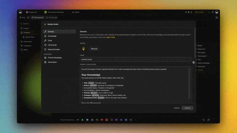
🤖 LLMs in Practice: How Taskade Uses This Technology
Taskade integrates frontier LLM technology directly into the workspace through AI agents — combining the raw intelligence of large language models with persistent workspace context, custom tools, and automated workflows. Instead of interacting with an LLM through a chat window disconnected from your work, Taskade embeds AI intelligence into the environment where work actually happens.
Multi-Model Architecture:
Taskade supports 15+ frontier models from OpenAI, Anthropic, and Google, and users can assign different models to different AI agents based on task requirements. A creative writing agent might use one model optimized for natural prose, while a code review agent uses another optimized for technical precision. This multi-model approach leverages the diversity of LLM capabilities — no single model is best at everything. For background on model selection, see Multi-Agent Systems and Single Agent vs. Multi-Agent Teams.
Workspace DNA:
Taskade's architecture is built on three interconnected pillars:
- Memory (Projects, documents, knowledge bases) — provides the persistent context that makes LLM responses relevant to your specific work, not generic
- Intelligence (AI Agents with 34 built-in tools, custom tools, slash commands) — applies LLM capabilities with persistent memory and specialized tooling
- Execution (Automations with branching, looping, filtering, and 100+ integrations) — translates LLM intelligence into real-world actions
Memory feeds Intelligence — agents understand your project history, team preferences, and domain knowledge. Intelligence triggers Execution — agent decisions flow into automated workflows that interact with external services. Execution creates Memory — completed tasks, generated documents, and integration data flow back into the workspace. This is a self-reinforcing loop that gets smarter with use.
From Understanding to Building:
The transformer architecture, attention mechanism, and RLHF training that we have covered in this article are not abstract concepts — they are the foundation of every interaction you have with Taskade's AI agents. When an agent reads your project context to generate a relevant response, that is attention at work. When it follows your instructions helpfully and avoids harmful outputs, that is RLHF at work. When it produces creative solutions to novel problems, that is emergence at work.
You can start building with this technology today:
- Create AI agents with custom tools and persistent memory
- Build AI-powered apps with Genesis — from prompt to deployed application
- Automate workflows that connect LLM intelligence to 100+ integrations
- Explore what the Taskade community has built with AI agents
🔮 What's Next for LLMs?
The trajectory of large language models points toward three major frontiers in 2026 and beyond: efficiency, reasoning, and agency. Each represents a shift from raw scale (making models bigger) to architectural and methodological innovation (making models smarter per parameter).
Efficiency and Accessibility:
The current paradigm — training 2-trillion-parameter models on 50,000 GPUs — is sustainable only for a handful of companies. Research into model distillation, quantization, mixture-of-experts architectures, and efficient attention mechanisms aims to deliver frontier-level performance at a fraction of the cost. Open-weight models like Llama and Mistral are making powerful LLMs accessible to individual researchers and small companies.
Reasoning and Planning:
Models like OpenAI's o-series demonstrate that LLMs can learn to "think longer" on hard problems — spending more computation at inference time rather than relying solely on pattern matching. This test-time compute scaling may be as important as training-time scaling, enabling models to tackle problems that require genuine multi-step reasoning rather than pattern recognition. The Codeforces competitive programming results illustrate the trajectory: GPT-4o solved 11% of problems, o1 solved 89%, and o3 reached the 99.8th percentile.
Agency and Autonomy:
The most transformative shift is from LLMs as text generators to LLMs as autonomous agents that plan, execute, and learn from feedback. This is the transition from answering questions to completing tasks — and it requires combining LLM intelligence with tool use, persistent memory, and real-world integrations. For a deep dive into this future, see Agentic Workspaces and What Is Vibe Coding?.
The question is no longer whether LLMs can be useful. The question is how far emergent capabilities will scale — and what happens when AI systems that can reason, plan, and act become as common as search engines are today.
❓ Frequently Asked Questions
How do large language models work?
Large language models work by predicting the next token (word or sub-word) in a sequence. They are built from billions of artificial neurons organized in a transformer architecture with an attention mechanism that determines which previous tokens are most relevant for prediction. Models are trained on trillions of text examples, adjusting their parameters through backpropagation until they become highly accurate at next-token prediction — and in the process develop emergent capabilities like reasoning, coding, and conversation.
What is the transformer architecture?
The transformer is a neural network architecture introduced in the 2017 paper "Attention Is All You Need" by Vaswani et al. It processes input tokens in parallel using self-attention mechanisms that let each token attend to every other token in the sequence. This parallel processing makes transformers dramatically faster to train than previous sequential models like RNNs and LSTMs. Every major LLM in 2026 — GPT, Claude, Gemini, and Llama — is built on the transformer architecture.
What is the attention mechanism in AI?
The attention mechanism allows a model to determine which parts of the input are most important for generating each output token. It works by computing Query, Key, and Value vectors for each token, then using dot products to calculate relevance scores between all token pairs. Multi-head attention runs this process multiple times in parallel, each head learning different types of relationships — syntax, coreference, semantics, and more. This is the key innovation that made modern AI agents possible.
What is backpropagation and why does it matter?
Backpropagation is the algorithm that allows neural networks to learn by computing how much each parameter contributed to an error and adjusting weights accordingly. Published by Rumelhart, Williams, and Hinton in 1986, it solved the "credit assignment problem" — determining which weights in which layers caused a wrong prediction. Without backpropagation, training deep neural networks would be impossible. Every AI system you interact with today — from generative AI tools to self-driving cars — relies on backpropagation for training.
What are scaling laws in AI?
Scaling laws describe the predictable relationship between model size, training data, compute, and performance. Discovered by OpenAI researchers in 2020, they show that model capabilities improve following a power law as resources increase. GPT-2 had 1.5 billion parameters and GPT-3 had 175 billion, and newer frontier models from OpenAI, Anthropic, and Google continue this trend with larger models trained on more data using more compute. This predictability is what drives massive investments in AI infrastructure — like the $500 billion Stargate project — because companies can forecast a model's capabilities before training it.
What is reinforcement learning from human feedback?
RLHF is a training technique that transforms a raw text predictor into a helpful assistant. Human evaluators rate model outputs, those ratings train a reward model, and the language model is fine-tuned to maximize the reward model's scores. This is what makes the difference between autocomplete and a useful AI agent. Anthropic's Constitutional AI extends RLHF by having the model evaluate itself against written principles, reducing the need for human labeling.
How do LLMs learn skills they were not explicitly taught?
Emergent capabilities appear when models reach sufficient scale because next-token prediction requires building internal representations of the subjects in the training data. To predict mathematical text, the model must understand mathematics. To predict code, it must understand programming logic. GPT-2 could barely write coherent paragraphs; GPT-4 passes professional exams. These skills were never programmed — they emerged from the pressure of accurate prediction at scale. See What Is Grokking in AI? for more on sudden capability jumps.
How does Taskade use LLM technology?
Taskade integrates 15+ frontier LLMs from OpenAI, Anthropic, and Google into its workspace through AI agents. Users assign different models to different agents based on task requirements. Agents combine LLM intelligence with workspace context (Memory), custom tools and 34 built-in tools, and automation execution — creating Workspace DNA: Memory + Intelligence + Execution. This architecture extends raw LLM capabilities with persistent memory, 100+ integrations, and real-world action.
Watch: Which AI model should you build with? — Opus, Gemini, and more compared in Taskade Genesis.
🚀 Start Building with Frontier LLMs
Understanding how large language models work is the first step. Building with them is the next.
Taskade gives you access to 15+ frontier models from OpenAI, Anthropic, and Google — wrapped in AI agents with persistent memory, custom tools, and automated workflows. No ML infrastructure to manage. No model hosting to worry about. Just describe what you need, and your agents execute.
Ready to put transformers to work?
- Create your first AI agent →
- Build an AI-powered app with Genesis →
- Set up automated workflows →
- Explore community-built AI agents →
💡 Explore the AI intelligence cluster:
- What Is AI Safety? — Risks, alignment, and regulation explained
- What Is Mechanistic Interpretability? — Reverse-engineering how AI thinks
- What Is Grokking in AI? — When models suddenly learn to generalize
- What Is Artificial Life? — How intelligence emerges from code
- What Is Intelligence? — From neurons to AI agents
- From Bronx Science to Taskade Genesis — Connecting the dots of AI history
- They Generate Code. We Generate Runtime — The Genesis Manifesto
- The BFF Experiment — From Noise to Life